
Scope
Here, we will apply the RFM model. An acronym for Recency, Frequency and Monetary, it is one of the easiest and most effective clustering models that can be applied to transactional data.
We will apply the model to two different datasets:
- CDNow contains customer transactions from CDNow, an e-commerce website focused on compact discs and music products. Click here for more information
- DonorsChoose.org is a non-profit organization, where it is possible to donate directly to state school projects. Click here for more informatio
The model requires the following data:
- The customer ID.
- The transaction date.
- The purchase amount.
Datasets Summary Statistics
A. CDNow
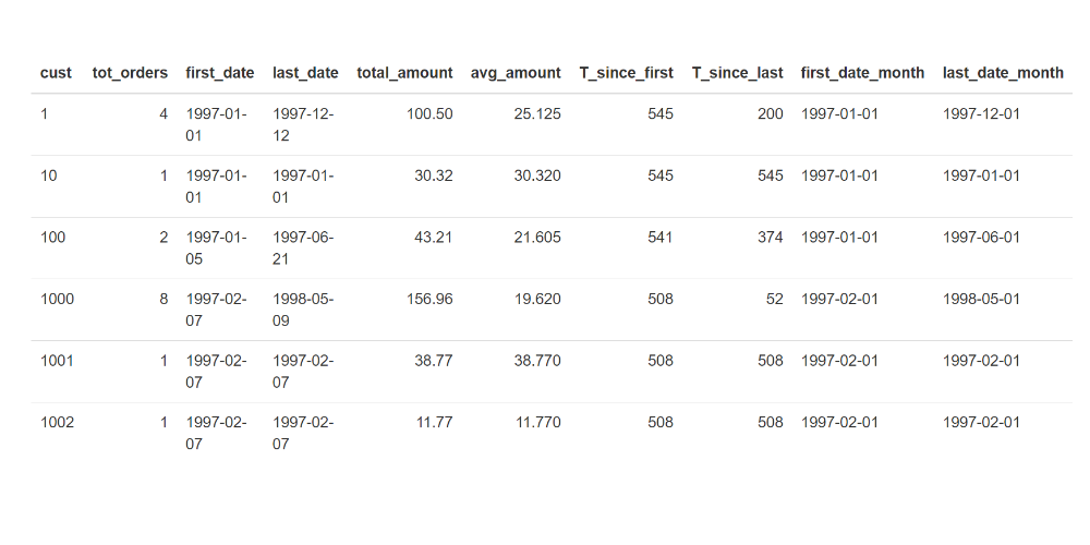
Below you can find some lines from the supplied dataset.
First lines of the CDNow dataset:
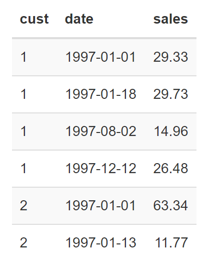
Where cust is the customer_id, date is the transaction date and sales is the total purchase amount.
Below you can see some figures from the dataset:
- Number of receipts: 6919
- Number of customers: 2357
- Number of receipts / number of customers: 2.94
- First transaction date: 1997-01-01
- Last transaction date: 1998-06-30
- Average transaction value: $35.28
Since we are concerned with customers’ purchase behavior, it is interesting to calculate some KPIs for each customer:
cd_today = max(cd_orders$date)

cd_customers_stats <- cd_orders %>%
  group_by(cust) %>%
  summarize(
    tot_orders = n(),
    first_date = min(date),
    last_date = max(date),
    total_amount = sum(sales),
    avg_amount = mean(sales)
  ) %>% mutate(
    T_since_first = as.numeric( difftime(cd_today, first_date, units = "days" ) ),
    T_since_last  = as.numeric( difftime(cd_today, last_date, units = "days" ) )
  )
Where tot_orders is the total number of orders, total_amount is the total purchase amount, avg_amount is the average expenditure, first/last_date is the first and last purchase date, T_since_first/last is the number of days between the first and last purchase (note that the chosen timeframe – cd_today – corresponds to the last date available in the dataset).
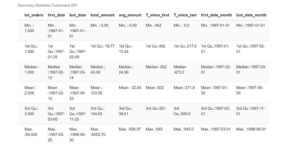
From the variable statistics, we can see that half of the population has made just one purchase, and the average expenditure is about $32. Furthermore, no new customer has been registered since 1997-03-25.
B. DonorsChoose.org
Below you can find some lines from the supplied dataset.

Below you can see some numbers about the dataset:
- Number of donations: 4687884
- Number of donors: 2024554
- Number of donations/number of donors: ** 2.32 **
- First donation date: 2012-10-08
- Last donation date: 2018-05-09
- Average donation value: $60.67
Since we are concerned with donor behavior, it is interesting to calculate some KPIs:
donation_today = max(donations$date)

donation_donors_stats <- donations %>%
                            group_by(`Donor ID`) %>%
                            summarize(
                              tot_donations = n(),
                              first_date = min(date),
                              last_date = max(date),
                              total_amount = sum(`Donation Amount`),
                              avg_amount = mean(`Donation Amount`)
                            ) %>% mutate(
                              T_since_first = as.numeric( difftime(donation_today, first_date, units = "days" ) ),
                              T_since_last  = as.numeric( difftime(donation_today, last_date, units = "days" ) )
                            )
Where tot_donations is the total number of donations, total_amount is the total amount donated, avg_amount is the average donation, first/last_date is the first and the last donation date, T_since_first/last is the number of days between the first/last donation (note that the chosen timeframe – donation_today – corresponds to the last date available in the dataset).
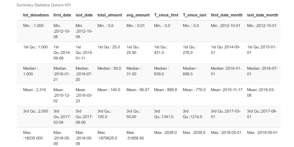
From the variable statistics, we can see that half of the population has made just one donation, and the average donation is around $56. There are also new donors close to the end of the available time frame.
Exploratory Data Analysis
In this section, we compare the two datasets.
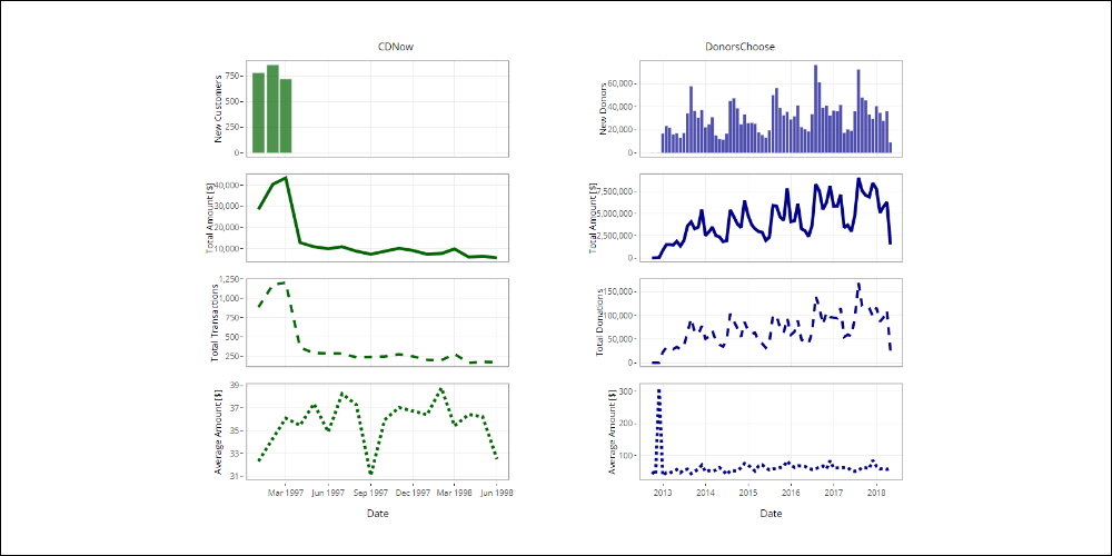
Time trends
Let’s start by exploring the transactions/donations over time. In the following plots, we show the total expenditure, the number of transactions/donations and the average spend per month.
Click the image below to navigate the graphic.
CDNow
- Let’s start by exploring the transactions/donations over time. In the following plots, we show the total expenditure, the number of transactions/donations and the average spend per month.
DonorsChoose
- A growing trend with visible seasonal cycles.
- The minimum values are close to June, the maximum close to August and December.
- The peak is in December 2012 and is due to a few but generous initial donations.
Customers/Donors distribution
To identify some behavioral patterns, we can explore the customers/donors distribution against certain variables.
Some of the most important variables are the Recency of the last purchase, the Frequency and the Monetary value (meaning the total expenditure).
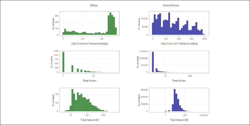
Click the image below to navigate the graphic.
Values
According to customer distribution for the Recency, Frequency and Monetary values, we have to assign a score to each customer’s variable, based on their behavior.
To calculate the scores, we use the quantiles and suppose that the grading scale ranges from 1-5.
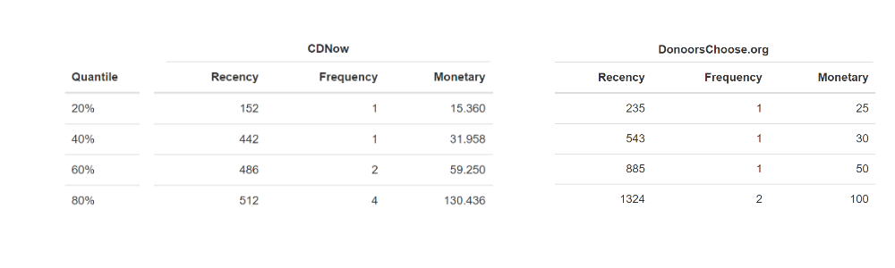
Below is the distribution for Recency, Frequency and Monetary with the respective quantiles for both datasets:
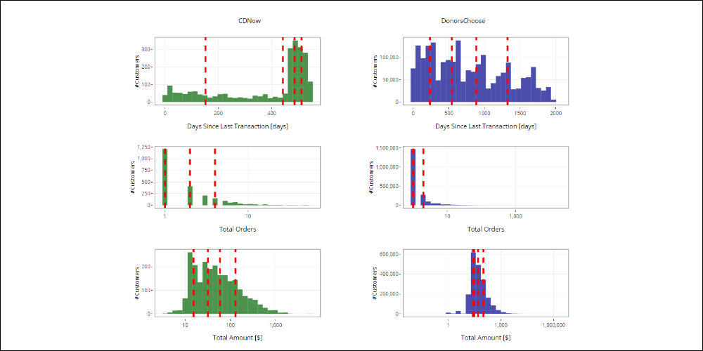
Click the image below to navigate the graphic.
From the previous tables we see:
- CDNow, In the case of frequency, the first and the second quantile are the same.
- DonorsChoose, In the case of frequency, the first, second and third quantile are the same.
In this case, we don’t have four different quantile values at our disposal, but rather some coinciding quantiles. To continue with assigning scores, we can do the following:
- Change the score scale (For example, assign scores between 1-3. From the earlier tables, we know there are at least 2 different tertile values for all the variables.)
- Do not assign some scores (For example, in the case of the CDNow frequency, we could choose not to assign the score of 5.)
In the following, you can see how it works, by using the second alternative. To use the first option, simply recalculate the corresponding quantiles.
For every client, we have to evaluate the range in which their Recency, Frequency and Monetary values fall and assign them the corresponding score values. Starting from the cd_customers_stats dataframe:
it is enough to compare the Recency, Frequency and Monetary value for each customer, with the thresholds found by the quantiles, then assign the scores accordingly:
#
# cd_customers_stats$Recency_score <- with(cd_customers_stats, ifelse(T_since_last <= 152, 5,
#                                                                     ifelse(T_since_last > 152 & T_since_last <= 442, 4,
#                                                                            ifelse(T_since_last > 442 & T_since_last <= 486, 3,
#                                                                                   ifelse(T_since_last > 486 & T_since_last <= 512, 2, 1)))))

cd_recency_threshold <- unique(cd_qnt_recency)
cd_customers_stats$Recency_score <- cut(cd_customers_stats$T_since_last, breaks = c(-Inf, unique(cd_recency_threshold), Inf), ordered_result = T)
cd_customers_stats$Recency_score <- as.integer(
  factor(
    cd_customers_stats$Recency_score_prova, levels = rev(levels(cd_customers_stats$Recency_score_prova))))

cd_frequency_threshold <- unique(cd_qnt_frequency)
cd_customers_stats$Frequency_score <- as.integer(cut(cd_customers_stats$tot_orders, breaks = c(-Inf, unique(cd_frequency_threshold), Inf),ordered_result = T) )

cd_monetary_threshold <- unique(cd_qnt_monetary)
cd_customers_stats$Monetary_score <- as.integer(cut(cd_customers_stats$total_amount, breaks = c(-Inf, unique(cd_monetary_threshold), Inf), ordered_result = T))
The Frequency and Monetary scores are calculated in the same way.
Time-based evolution of quantiles
The use of quantiles allows the thresholds that are selected for every Recency, Frequency and Monetary variable to adapt to the natural evolution of the data. This ensures a cluster definition that is consistent with the available information.
Below we show the first and fourth quantile for each Recency, Frequency and Monetary variable over time.
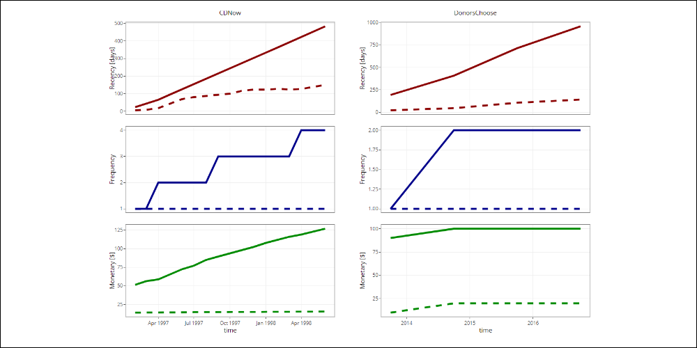
Click the image below to navigate the graphic.
RFM cube
Calculating the Recency, Frequency and Monetary scores is equivalent to mapping the three variables to a cube that has the same dimensions as the chosen value scale.
Here are the two RFM cubes:
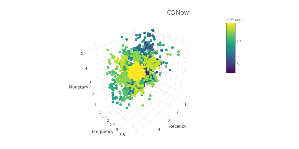
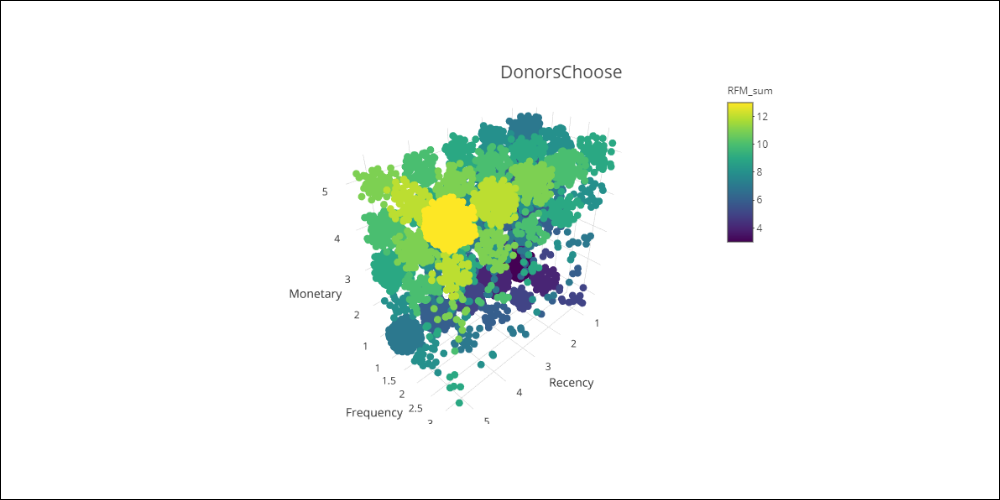
Click the images below to navigate the graphics.
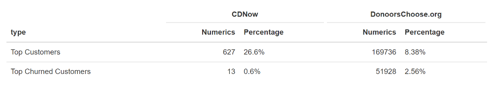
Top Customers and those at risk of churning
By selecting specific Recency, Frequency and Monetary scores, we can define the top customers and those at risk of churning.
In the case of CDNow, we can select the following scores to identify the two most important purchase behavior patterns:
- Top Customers: R = 4-5,F = 3-4, M = 4-5
- Top Churned Customers: R = 1-2, F = 3-4, M = 4-5
The identified Churn Customers are those who had high spending levels and bought frequently, but who have not purchased anything for a long time (R = 1-2).
In the case of DonorsChoose:
- Top Customers: R = 4-5,F = 3, M = 4-5
- Top Churned Customers: R = 1-2, F = 3, M = 4-5
The results are shown below:
Can we use RFM as a simple predictive model?
In this section, we want to test how effective the RFM model is. In particular, we want to understand how valid the concept is, of selecting top customers and those who are at risk churning. For example, by selecting the top customers, we are implicitly assuming that they will remain so in the future.
We can test this assumption by setting a past time frame that defines a period that can be used to determine the behavior of customers by assigning the relevant scores, and a ‘future’ period, which can be used to check whether the top customers have remained as such.
The two analyzed datasets have a different time frame and for this reason, we choose:
CDNow:
- calibration: 1 year
- test: 6 months
DonorsChoose:
- Calibration: 4 years
- Test: 2 years
Below are the trends for new customers/donors and their total expenditure/total donations per month, in relation to the chosen time frame in each case. In the following analysis, the customers/donors who purchased/donated after the chosen time frame are not considered.
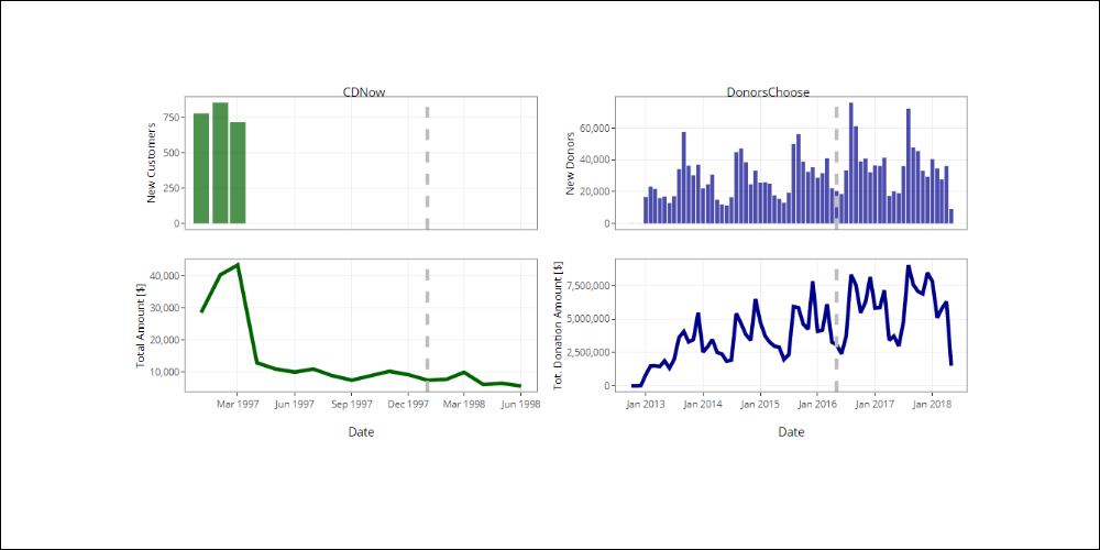
To measure the accuracy of the RFM assumptions, we have recalculated the scores during the calibration period, and have only considered the Top Customers and the Top Churned Customers, as defined by the previously expressed rules.
We have also verified the behavior of both the Top Customers and the Top Churned Customers in the future period. The goal is to understand the value of assumptions such as ‘The Top Customers will continue to be top customers’, or ‘Customers I consider to be Top Churn Customers will really behave that way’.
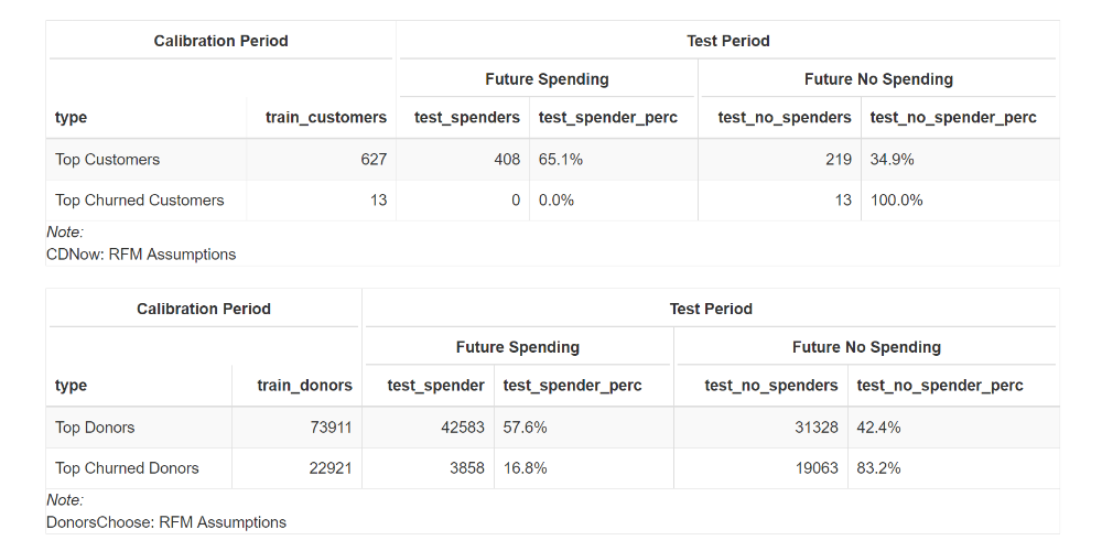
The following tables show the numbers for both types of customer in comparison with the future period, and in particular, whether they made a purchase/donation or not during this period.
In the case of CDNow:
- 65% of those who were Top Customers during the calibration period, continued to buy in the following period.
- 35% of those who were Top Customers during the calibration period, didn’t continue to buy in the following period.
- 100% of those who were Top Churned Customers during the calibration period, were customers who really churned.
In the case of DonorsChoose:
- 57.6% of those who were Top Donors during the calibration period, continued to donate in the following period.
- 42.4% of those who were Top Donors during the calibration period, didn’t keep on donating in the following period.
- 83.2% of those who were Top Churned Donors of the calibration period, actually stopped donating.
- 16.8% of those who were Top Churned Donors during the calibration period, returned to donate again.
We have tested, as a result, the implicit RFM model assumptions.
For both datasets, the Top Churned prediction is more accurate, with the Recency variable being very important to both the music and donation sectors. With regard to the ‘Top Customers will continue to be top customers’ assumption, approximately 40% of the Top Customers in the calibration period didn’t buy or donate in the future period, which indicates a sizeable limitation for use as a predictive model. We need to remember that approximately 20% of the top spender customers generate roughly 80% of revenues. As a result, assuming that the Top Customers will remain as such, without investigating an alternative strategy, could be very dangerous. As the figures show, approximately 40% of the top customers did not, in fact, maintain their status.
However, it is important to point out that the RFM model was created as a clustering model based on actual data. It defines a realistic view of the database and its clusters, made up of everyone from top customers, to those at risk of churn.
Conclusions
We have applied the RFM model (Recency, Frequency and Monetary) to two datasets, CDNow from the field of music and DonorsChoose.org, a charitable organization. The applied model gives a score to customer/donor spending behavior, and so creates clusters from the database. In particular, we have shown a potential categorization of Top Customers, those who recently spent a lot, with a high frequency, and the Top Churned Customers, meaning those with a high value but who have probably churned.
By identifying behavioral purchase patterns, it is possible to apply custom strategies to each cluster, such as retention activities for the customers who are at risk of churning, loyalty programs for top spenders and up-selling campaigns for customers with a middle-low purchase level, who can be seen as not being loyal. For example, a Recency of 3, a Frequency of 1-2 and a Monetary value of 2-3.
Are you curious to use the RFM in your business? Here you can find some suggestions.